APIs are contracts. Once clients depend on one, every careless choice becomes permanent — you can add almost anything, but you can remove almost nothing. These twelve concepts are the difference between an API that scales gracefully and one that becomes the bottleneck in every meeting.
The three conversation styles
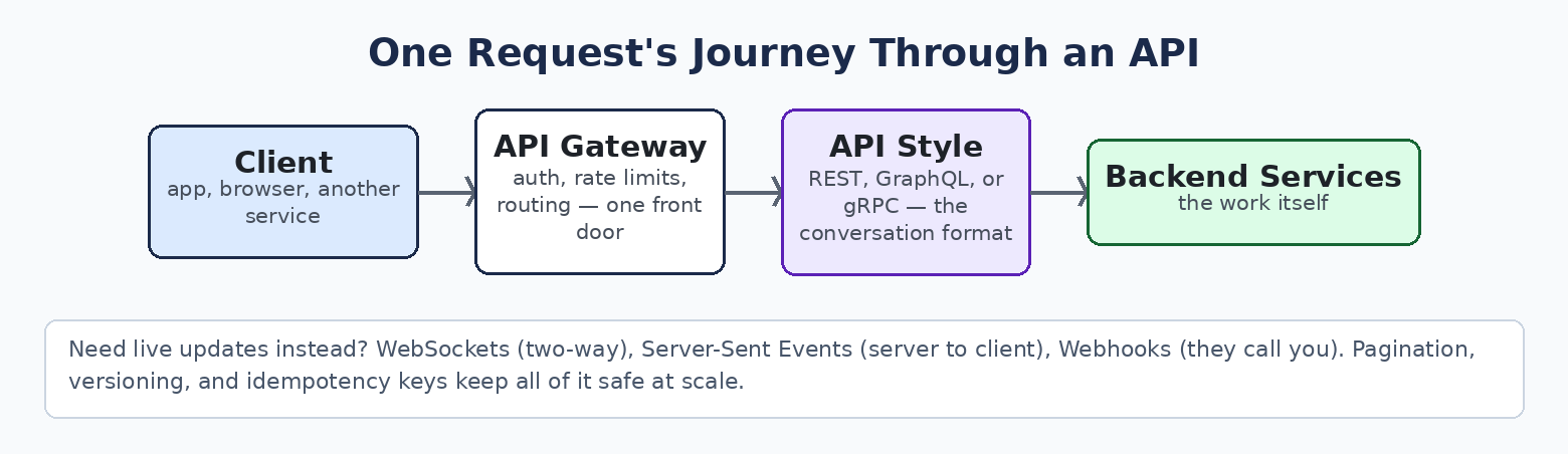
1. REST. Resources as URLs, acted on with HTTP verbs: GET /orders/42 reads one, POST /orders creates one, PUT replaces, DELETE removes. It is the default because it is simple, cacheable, and every developer alive already speaks it.
2. GraphQL. One endpoint; the client sends a query naming exactly the fields it wants, and gets exactly those back — no more, no less. It ends over-fetching and under-fetching, and it shines when many different clients (web, iOS, Android) need different shapes of the same data.
3. gRPC. Remote function calls over HTTP/2 using Protobuf — a compact binary format with a strict contract. Faster and smaller than JSON, made for service-to-service traffic inside your system, where browsers are not involved.
Rule of thumb: REST for public APIs, GraphQL for client-driven data needs, gRPC between your own services.
The three ways to push
4. WebSockets. One connection, upgraded from HTTP, kept open for messages in both directions. Chat, live dashboards, games — anything where the client also talks back constantly.
5. Webhooks. The provider calls your URL when something happens: payment completed, build finished, shipment moved. They call you, so you never poll. If your design has a loop asking “is it ready yet?”, a webhook probably deletes it.
6. Server-Sent Events (SSE). A one-way stream from server to client over plain HTTP. Simpler than WebSockets when the client only listens — notifications, feeds, and the token-by-token streaming of LLM responses, which is exactly how most AI chat products work under the hood.
The five that keep you safe at scale
7. Pagination. Never return a list unbounded. Return a page (say 20 items) plus a cursor pointing at the next page. Cursors beat page numbers because they stay correct while data changes underneath.
8. Rate Limiting. A cap per client per window — 100 requests a minute, say. Under the limit, requests pass; over it, a 429 and a “retry later.” It protects the service from abuse, accidents, and any single customer becoming everyone’s outage.
9. Idempotency Keys. The client attaches a unique key to a request. First arrival: do the work (charge the card), save the result against the key. A retry with the same key: skip the work, return the saved result. This one header is what makes retries — and payments — safe.
10. Versioning. Ship breaking changes as /v2/ while /v1/ keeps running, retire v1 only when clients have migrated. Versioning is how an API evolves without breaking the people who trusted it.
11. OAuth / JWT. OAuth handles permission (a user lets an app act on their behalf); the JWT is the signed token that proves who is calling and what they may do, checked by the API on every request without a database lookup.
12. API Gateway. One entry point in front of many services: authentication, rate limits, routing, and logging in a single place, so every service behind it does not reinvent them. Clients see one door; you operate a building.
The bottom line
Pick the conversation style by who is talking (public, client-driven, or internal), the push mechanism by direction (both ways, event-driven, or listen-only), and treat pagination, rate limiting, idempotency, versioning, and the gateway as non-negotiable from day one. Retrofitting any of them costs ten times what designing them in does.
Building APIs or AI platforms that have to survive production? The free architecture toolkits go one layer deeper.
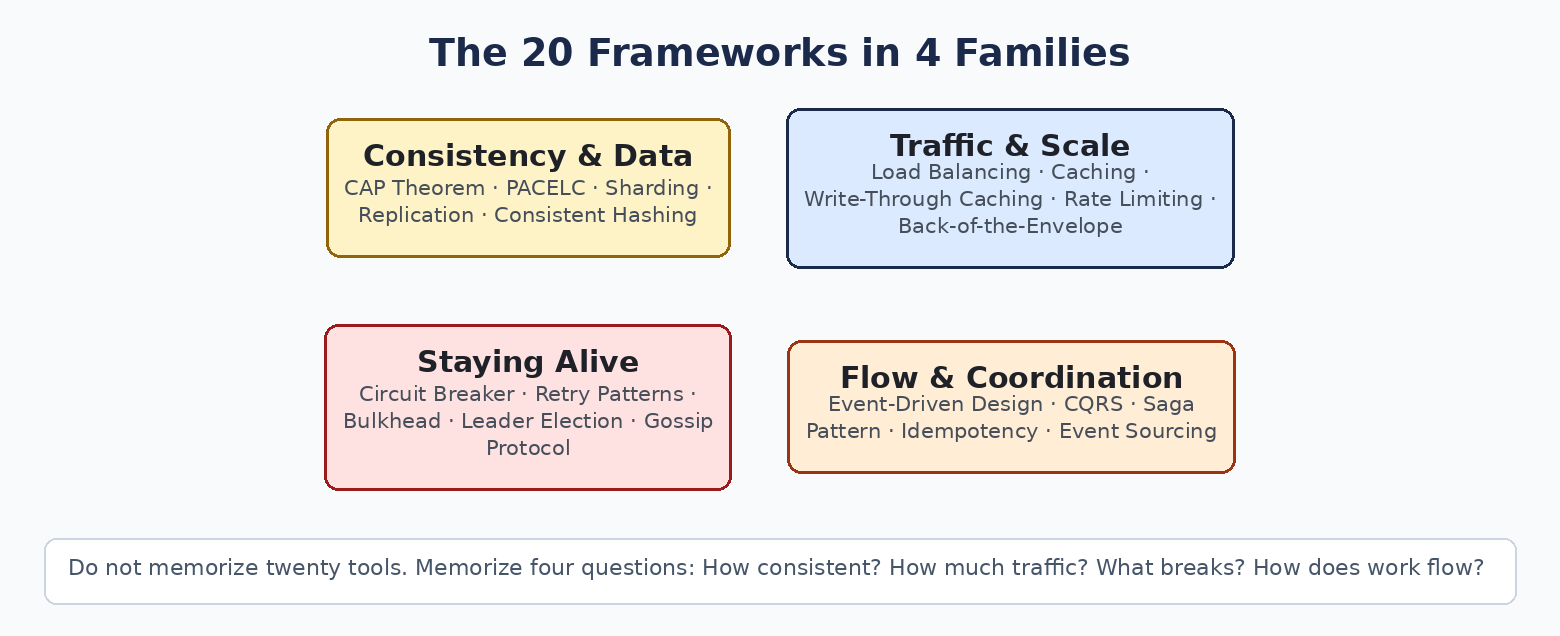
Twenty frameworks is a lot to memorize — until you notice they are answers to only four questions. How consistent must the data be? How much traffic is coming? What happens when something breaks? And how should work flow between services?
Sort the twenty into those four families and the list stops being a list. It becomes a checklist you can run in any design review.
Family 1: Consistency & Data — “What is the truth, and where does it live?”
CAP Theorem. When a network partition splits your system, you must choose: stay consistent (every read sees the latest write) or stay available (every request gets an answer, possibly stale). You cannot have both during a partition. This is the first fork in every distributed design.
PACELC Model. CAP only speaks during failures. PACELC adds the everyday case: else (no partition), you still trade Latency against Consistency. It is CAP for real life, because most days nothing is broken — and you are still making the trade.
Database Sharding. Split one large dataset across many databases — by user ID, by region, by any key that spreads the load evenly. Reach for it when a single database genuinely cannot carry the workload, not before.
Replication. Copy data across nodes so the system survives losing one. Leader–follower when one writer is enough; multi-leader when writes must happen in more than one place. Replication buys reliability and read scale; it charges you in consistency headaches.
Consistent Hashing. The ring that decides which node owns which key — designed so that adding or removing a node moves only a small slice of the data, not everything. It is why sharded systems can scale without a weekend of rebalancing.
Family 2: Traffic & Scale — “Too many requests, not enough server”
Load Balancing. Spread incoming traffic across servers: round-robin for simple cases, least-connections when requests vary, hashing when a user must land on the same node. The goal is boring — no server drowning while its neighbor idles.
Caching Strategies. Keep frequently read data close and fast. Cache-aside (the app checks the cache, fills it on a miss), write-through, write-back — the variations are about when the cache and the database agree.
Write-Through Caching. The specific pattern worth naming on its own: every write updates the cache and the database together, so the cache is never stale. You pay a little write latency to buy reads you can trust.
Rate Limiting. Cap how many requests a client may make in a window. It protects availability, enforces fairness between customers, and turns abuse into a polite 429 instead of an outage.
Back-of-the-Envelope Estimation. Rough capacity math with stated assumptions: users × requests × size = storage, bandwidth, servers. Five minutes of arithmetic that kills unbuildable designs before they consume a quarter.
Family 3: Staying Alive — “Something will fail; then what?”
Circuit Breaker. When a downstream service keeps failing, stop calling it for a while — fail fast, let it recover, test it with a trickle before reopening the floodgates. Named after the electrical part because it does the same job: it keeps a fault from burning down the house.
Retry Patterns. Failed requests often succeed on a second attempt — but retry with exponential backoff and jitter, or a thousand clients retrying in lockstep become the outage.
Bulkhead Pattern. Partition your own resources the way a ship’s hull is partitioned: separate thread pools per dependency, so one slow service floods only its own compartment instead of sinking the whole application.
Leader Election. In a cluster, exactly one node coordinates. Leader election picks that node dynamically and replaces it when it dies — the quiet mechanism behind half the systems in this list.
Gossip Protocol. Nodes spread state by chatting with random peers, the way news spreads through an office. No central coordinator, no bottleneck — large clusters stay informed eventually, which is usually enough.
Family 4: Flow & Coordination — “How does work move and stay correct?”
Event-Driven Design. Services react to events instead of calling each other directly. The producer does not know or care who consumes — which is what decoupling actually means.
CQRS. Separate the write model from the read model (Command Query Responsibility Segregation). When reads and writes have wildly different shapes and volumes, optimizing one shared model serves neither.
Saga Pattern. A distributed transaction built from local transactions plus compensating actions. Book the flight, charge the card, reserve the hotel — and if step three fails, undo steps one and two. No two-phase commit across services; consistency by choreography instead.
Idempotency. Design operations so running them twice has the same effect as running them once. It is what makes retries, duplicate deliveries, and nervous users with double-clicks safe — the foundation every payment API stands on.
Event Sourcing. Store the events (what happened) instead of the final state. Current state is rebuilt by replaying history — which gives you a complete audit trail and time travel as side effects. Powerful, and heavier than most systems need.
The bottom line
Nobody recalls twenty frameworks under pressure. They recall four questions — consistency, traffic, failure, flow — and pull the right tool from the right family. Learn the families and the twenty names will attach themselves.
Want the whole set as a printable reference? The free toolkits at aideeva.com/free-toolkits/ include the AI Engineering Iceberg Poster and architecture cheat sheets built the same way — grouped to be remembered.
Every enterprise AI program hits the same architectural moment. The model is selected, the proof of concept impressed the room, and then somebody asks the production question: how do we serve this — at our volume, our latency targets, our cost ceiling?
That question is an architecture decision, and it deserves to be treated like one. The serving engine you choose determines your GPU economics (how many users one accelerator can carry), your latency profile (how fast the first token arrives under load, not in a demo), your scaling ceiling, and your operational burden for years. Choose on fashion and you will re-platform within two quarters. Choose on workload shape and the decision holds.
Three engines dominate the open-source serving conversation: Ollama, vLLM, and SGLang. They are usually compared as competitors. From an architect’s chair, they are better understood as three design centers — three different answers to three different traffic shapes:
Ollama is designed around a person — one developer, one machine, minimal surface area.
vLLM is designed around a crowd — high concurrency, mostly unique prompts, maximum throughput per GPU.
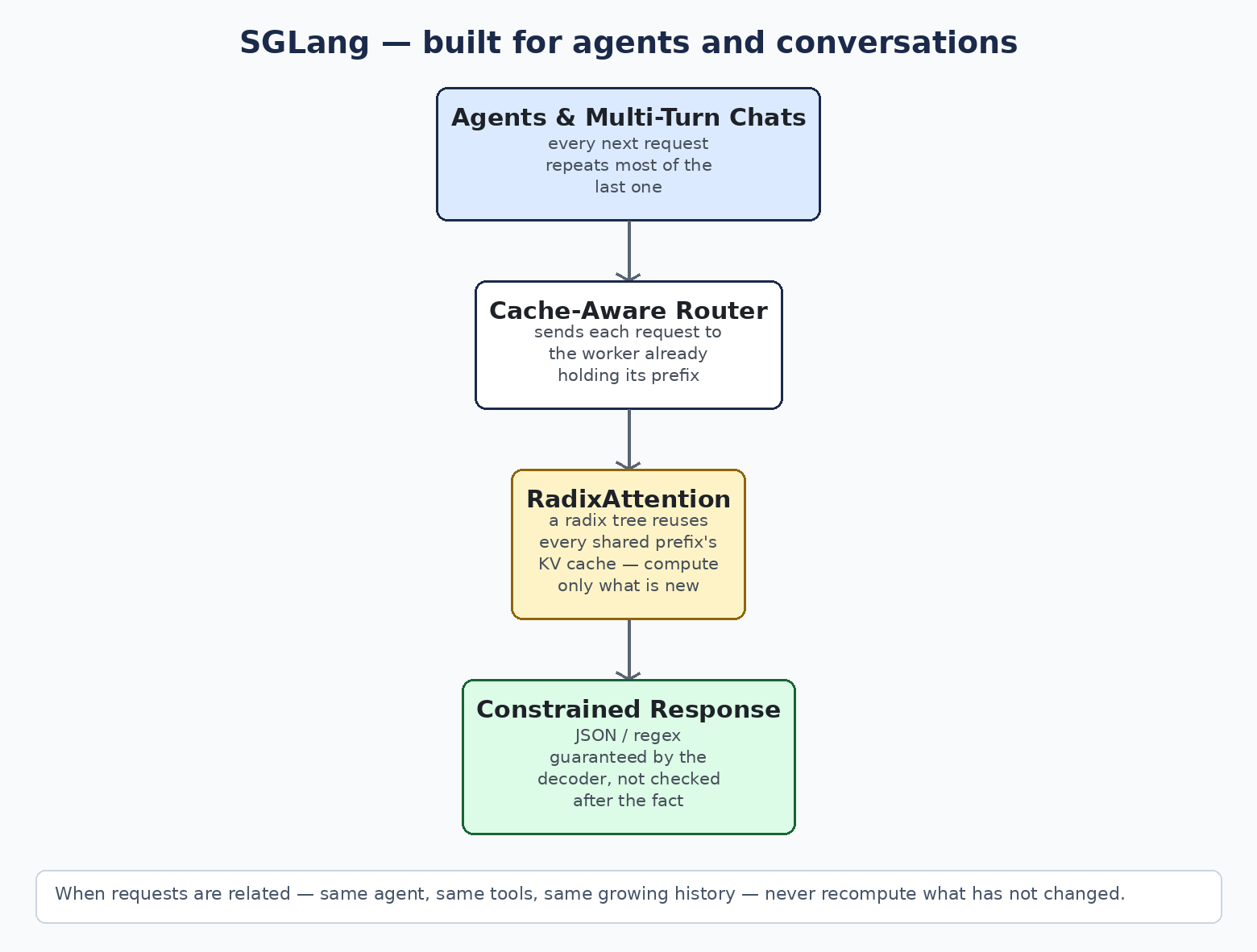
SGLang is designed around a conversation — agents and multi-turn systems whose requests share long, growing prefixes that should never be computed twice.
This deep dive works the way an architecture review should: the mechanics first, then each engine on its merits and limits, then the capacity math, the scaling patterns, the failure modes — and only then the recommendation.
The mechanics that decide everything
Serving economics are governed by a handful of mechanisms. Every claim in this article reduces to one of them.
Prefill and decode. Each request has two phases. Prefill processes the prompt — parallel, compute-heavy, done once. Decode generates the answer one token at a time, each step dependent on the last — sequential and memory-bandwidth-bound. Prefill cost scales with prompt length; decode cost scales with answer length and with how much state the engine must re-read at every step. Most serving optimization is an attack on one of these two phases.
The KV cache is the real capacity constraint. During generation, the model stores the attention keys and values for every token it has processed, so nothing is recomputed. This cache grows linearly with context length and with concurrent requests. In production, the KV cache — not the model weights — is usually what exhausts GPU memory first. How an engine allocates, shares, and evicts this cache is the single strongest predictor of how many users it can serve per GPU.
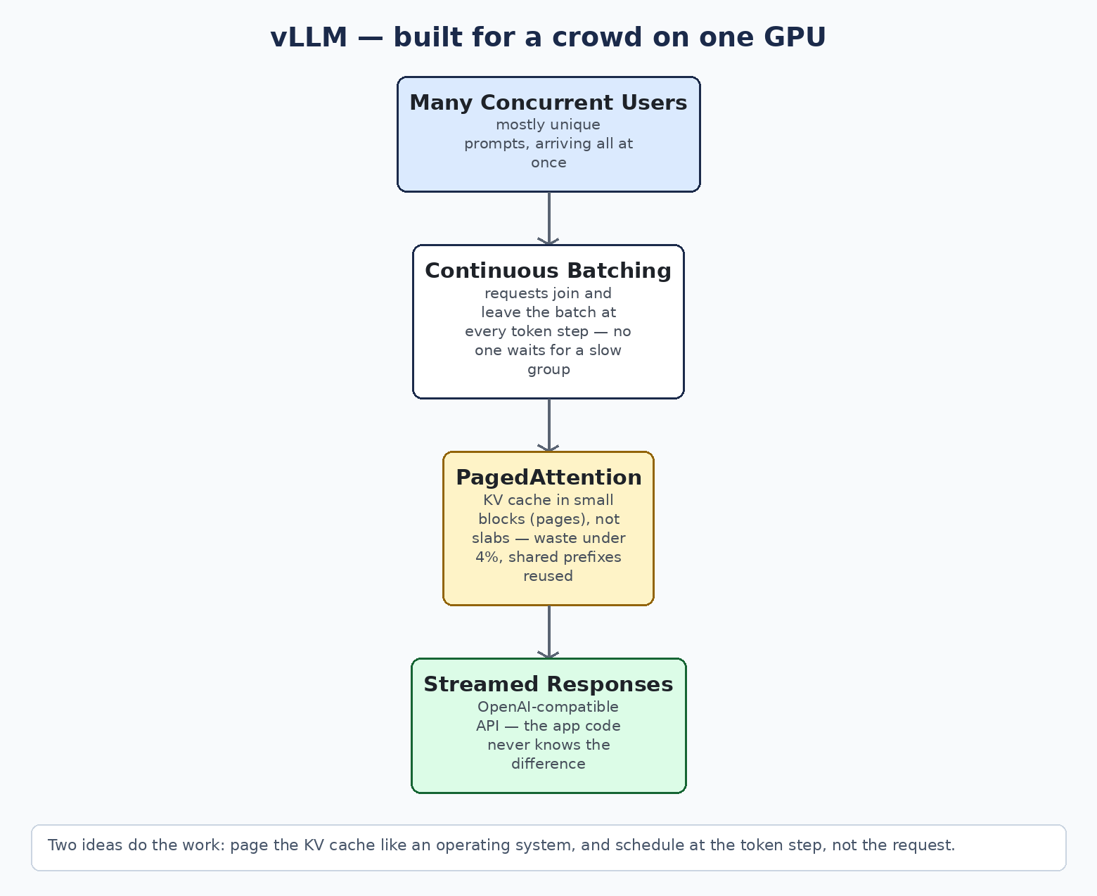
Batching, and why “continuous” changed the field. GPUs are throughput machines: processing 32 sequences together costs little more than processing one. Static batching assembles a fixed group and runs it to completion — one long generation stalls the entire group. Continuous batching (iteration-level scheduling) admits and retires requests at every token step: a finished request releases its slot instantly, a waiting one takes it. This is the mechanism behind the modern engines’ throughput advantage, and it is non-negotiable for multi-user serving.
Latency vs. throughput is a trade you make explicitly. The user-facing metrics are time-to-first-token (TTFT) and per-token latency under load; the business-facing metric is aggregate tokens per second per GPU, which is cost. Larger batches raise throughput and can raise individual latency. An architecture that does not state which side of this trade it is optimizing — interactive chat or overnight batch — is not finished.
Quantization moves the memory budget. Storing weights at 4-bit instead of 16-bit shrinks a model roughly four-fold, at a small quality cost. GGUF is the quantized format the local ecosystem standardized on. Quantization matters architecturally because every gigabyte not spent on weights is a gigabyte available for KV cache — which is to say, for users.
Prefix reuse is free throughput, if your traffic has prefixes. Requests that share a beginning — a system prompt, tool definitions, a conversation’s history — can reuse the KV cache computed for that beginning instead of recomputing it. The architectural question is never whether an engine caches prefixes; it is how granular the sharing is (whole blocks? branching trees?) and whether scheduling and routing cooperate to keep the cache warm.
Constrained decoding turns output contracts into guarantees. Forcing generation to obey a JSON schema, regex, or grammar — by masking invalid tokens during decode — converts “the model usually returns valid JSON” into “the output is valid by construction.” For agent pipelines and tool calling, this is the difference between a system and a hope.
1. Ollama — the developer-machine engine
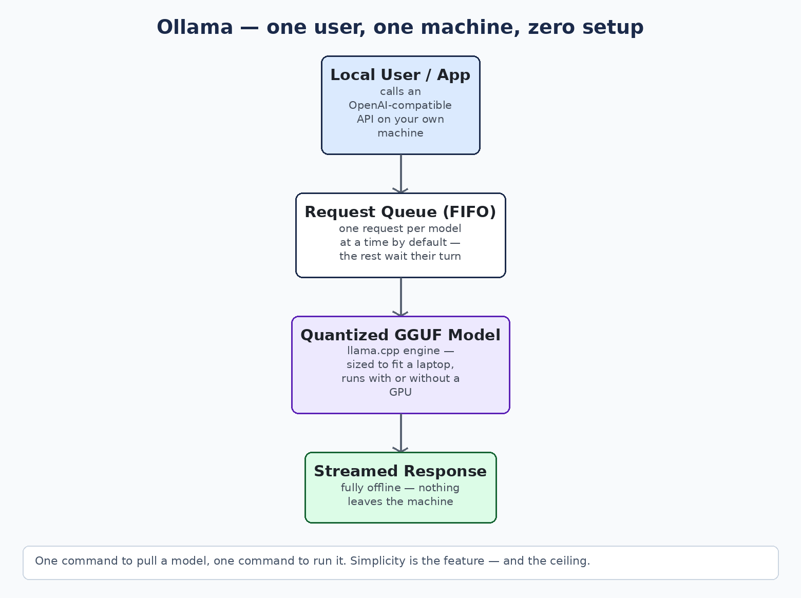
How it works. Ollama packages the llama.cpp inference engine behind a one-command experience: pull a quantized GGUF model, run it, call it over a local API (its own REST interface, plus an OpenAI-compatible endpoint). Requests to a model are queued and processed one at a time by default (OLLAMA_NUM_PARALLEL, default 1), with up to 512 requests waiting before the server starts returning errors. Models load on demand and unload after roughly five idle minutes. Everything runs locally and offline; hosted cloud models exist as an optional extra.
Where it earns its place. Developer workstations, proofs of concept, and genuinely small internal tools. Its architectural virtue is a tiny operational surface: no cluster, no tuning, no GPU fleet — a model running in minutes on a laptop, including machines with no discrete GPU. For data-residency-sensitive experimentation, “nothing leaves this machine” is a complete architecture, and Ollama delivers it with the least ceremony in the field. A large share of enterprise AI work starts here, and low-concurrency internal tools legitimately stay here.
Where it breaks. The design center is a single user. Raise the parallel setting and each slot multiplies reserved context memory; there is no continuous batching, so under real concurrency the queue — not the GPU — becomes the bottleneck, and latency grows linearly with arrivals while the hardware idles. There is no built-in authentication (it assumes a trusted local network), no multi-GPU serving story, and no meaningful observability surface for production SLOs. None of this is a defect; it is a boundary. The failure mode is ignoring the boundary — promoting a developer tool into a serving tier because it was already installed.
The architect’s verdict. Standardize on Ollama for the inner loop: development, evaluation, demos, and isolated single-user tools. Write the exit into the design from day one — code against the OpenAI-compatible endpoint, so promoting the workload to a production engine is a deployment change, not a rewrite.
2. vLLM — the production throughput engine
How it works. vLLM, out of UC Berkeley, is built on one diagnosis: legacy serving wasted most of the KV cache. Older systems reserved each request a contiguous slab of GPU memory sized for its maximum possible generation, and the vLLM paper measured that only a small fraction of the reservation ever held live data. PagedAttention applies the operating-system answer — paging. The KV cache is divided into small fixed-size blocks, allocated wherever memory is free, with a block table mapping each request’s logical sequence to physical blocks. Waste collapses to the tail of the final block — under 4% in the paper’s measurements — and the recovered memory converts directly into larger batches. Layered on top: continuous batching at the token step, prefix caching enabled by default in the current V1 engine, tensor and pipeline parallelism for models that exceed one GPU, and the broadest model and accelerator support in the open ecosystem, behind an OpenAI-compatible API.
Where it earns its place. The default production serving tier. Public and internal API platforms with many concurrent users and mostly unique prompts; enterprise chat and RAG front doors; and batch estates — document processing, enrichment, evaluation — where overnight throughput per dollar is the governing metric. When a capacity plan says “we must carry N concurrent sessions on M GPUs,” vLLM is the engine that makes the arithmetic work, and it is the baseline against which every alternative must benchmark.
Where it breaks. It is data-center infrastructure, with a data-center footprint: it assumes real GPUs (it is not a workstation tool), and by default it claims ~90% of GPU memory, which collides with shared-card environments. The tuning surface is real — memory utilization, max concurrent sequences, block size, chunked-prefill behavior — and rewards teams that load-test over teams that guess. Its prefix caching, while solid, is block-granular and designed for breadth; workloads whose traffic is dominated by long shared prefixes are precisely the shape the next engine was designed around. Operationally, you are adopting a fast-moving platform: version discipline and upgrade testing belong in the runbook.
The architect’s verdict. Make vLLM the reference architecture for shared, multi-user LLM serving unless the workload’s shape argues otherwise. Budget the engineering honestly — load testing, tuning, GPU capacity management — because the engine’s economics only materialize when it is operated as infrastructure, not installed as a package.
3. SGLang — the engine for agent and conversation traffic
How it works. SGLang, from the LMSYS team, starts from an observation about production agent traffic: requests in these systems are not independent. An agent’s fifteenth tool call carries the same system prompt, the same tool definitions, and the same accumulated history as its fourteenth — plus one delta. RadixAttention manages the KV cache as a radix tree keyed by token prefixes: an incoming request walks the tree, reuses every matching cached prefix — including branching, multi-level sharing across sessions that diverged from a common trunk — and computes only the new suffix. Unused branches are evicted LRU-style, so the cache behaves like a cache, not a leak. The scheduler is cache-aware: it orders work so requests sharing a prefix run while their shared branch is resident, and in multi-worker deployments its router directs each request to the worker already holding that prefix. Its constrained decoding compiles the output grammar into a compressed finite-state machine, allowing the decoder to advance through forced token stretches in jumps — structured output that is both guaranteed and fast. Continuous batching and the rest of the modern toolkit are present, as they now are everywhere.
Where it earns its place. Agent platforms and tool-calling loops, where each step resends a growing context and naive serving re-bills you for your own history at every step. Multi-turn chat at scale, where a conversation’s history is literally a prefix of its next request. Few-shot and self-consistency patterns, which are prefix-sharing by construction. RAG serving with long, stable system prompts and templates. In these shapes, prefix reuse is not a micro-optimization: it compounds with concurrency (more sessions share more of the tree) and flattens the cost curve that otherwise grows with conversation length.
Where it breaks. Remove the shared prefixes and you remove the thesis: on unique, unrelated prompts, SGLang performs comparably to vLLM, and you have adopted a specialist to do a generalist’s job. Its ecosystem — documentation depth, community answers at 2 AM, day-one support for exotic new models — is smaller than vLLM’s, which is a real operational cost that belongs in the decision record. Cache-awareness also introduces a systems subtlety: routing and scheduling now have state (where prefixes live), which complicates load balancing and failover design compared to stateless round-robin over identical workers.
The architect’s verdict. Where agent and multi-turn traffic is a first-class workload — not an experiment — SGLang is the architecturally correct answer, because it is the only one of the three whose core data structure matches the traffic’s shape. Pilot it against your real prompt distribution; the prefix hit-rate in your own telemetry is the number that justifies it.
Capacity planning: the math that sizes the decision
Engine selection is inseparable from sizing. The governing equation is simple to state:
Concurrency is bought with cache. A modest model serving fifty concurrent users at long context can require more memory for KV cache than for its weights. This is why PagedAttention’s waste elimination and RadixAttention’s sharing are economic features, not academic ones — every recovered gigabyte is headroom for sessions.
Quantization is a capacity lever, not just a quality trade. Halving weight precision frees memory that converts directly into concurrent sessions or longer contexts. Evaluate quantized variants against your quality bar explicitly; for many enterprise workloads the 4-bit/8-bit quality delta is smaller than the concurrency delta is valuable.
Prefix hit-rate is a capacity input. In agent estates, a high radix-cache hit rate reduces effective prefill — often the dominant compute — by the shared fraction. Two deployments with identical GPUs can differ several-fold in carried sessions purely on how much of each prompt was already cached. Measure your prompt-overlap distribution before you size anything.
A defensible capacity plan names: target concurrent sessions, p95 context length, target TTFT and per-token latency at that concurrency, and the resulting GPU count per engine. If a vendor or a blog gives you tokens-per-second without the concurrency and context it was measured at, it has given you marketing, not engineering.
Scaling patterns
Single node → multi-GPU. When a model exceeds one GPU, tensor parallelism shards it across devices; this is a serving-tier concern (vLLM and SGLang), never a workstation one. Treat interconnect bandwidth as part of the design — tensor parallelism is chatty.
Single replica → fleet. Scale-out adds a routing tier, and here the engines diverge architecturally. Stateless round-robin is simple and works acceptably for vLLM, though per-replica prefix caches mean shared prefixes get recomputed across the fleet. For SGLang-class workloads, cache-aware routing — directing a session to the replica holding its prefix — is the difference between the design working and the design merely running. Stateful routing buys hit-rate with failover complexity; make that trade consciously.
The gateway is not optional in production. None of these engines is a complete serving platform. The reference pattern wraps the engine tier with authentication and authorization, per-consumer rate limiting and quotas, request logging for audit, and metrics that matter: TTFT and latency percentiles, queue depth, KV-cache utilization, and prefix-cache hit rate. Ollama in particular ships no authentication — anything beyond a workstation must sit behind this tier.
Failure modes worth designing for
Cache exhaustion under load spike. Long contexts × a concurrency spike exhausts KV memory; engines queue or preempt. Design the degradation: bounded context windows, admission control, and honest 429/503 behavior beat silent latency collapse.
Prefix-cache thrash. If working-set prefixes exceed cache capacity, hit rates crater and latency regresses toward the no-cache case — a cliff, not a slope. Size the cache to the working set, and alert on hit rate, not just latency.
Queue saturation on the wrong engine. Ollama’s default — one in-flight request per model, queue of 512, then refusals — is a fine workstation contract and a production outage. This failure mode is a selection error, not a product defect.
Cold starts. Multi-gigabyte model loads and engine warm-up are minutes, not milliseconds. Autoscaling policies, pre-warmed replicas, and scale-to-zero decisions must be made against that reality.
Silent quality drift via quantization mismatch. A workload validated at full precision and deployed at 4-bit (the Ollama default) is a different system than the one you tested. Pin precision in the deployment record.
The part most comparisons get wrong
Feature matrices say these engines have converged, and at the checklist level they have: continuous batching, prefix caching, structured outputs, speculative decoding, and quantization are table stakes across the serious engines. Architects should be suspicious of checklist equivalence. What differs is design center, defaults, and the data structure at the core — a FIFO queue tuned for one user, a paged cache tuned for crowd throughput, a radix tree tuned for reuse across related requests. Benchmarks alternate winners between vLLM and SGLang because benchmarks have shapes: each engine wins the workload it was designed around. The professional question is never “which engine is fastest?” It is “what does my traffic actually look like — measured, not assumed — and which design center matches it?”
The second-order point is reversibility. All three engines expose OpenAI-compatible APIs, so the application layer can be insulated from the choice. Prototype on Ollama, launch the shared tier on vLLM, carve the agent estate onto SGLang — each step is a deployment migration, not an application rewrite. An engine decision with a tested exit is a low-risk decision; insist on the exit.
The decision guide
Your situation
Pick
Why
Developer inner loop: build, evaluate, demo
Ollama
Minimal operational surface; a model running in minutes, offline, on the machine in front of you
Data-residency-bound experimentation; single user or tiny team
Ollama
Local-first by architecture; nothing leaves the machine
Shared production API: many concurrent users, mostly unique prompts
vLLM
PagedAttention + continuous batching = the most carried sessions per GPU for crowd-shaped traffic
Aggregate throughput is the governing metric; the offline batch path is built for it
Enterprise chat / RAG front door with a mixed audience
vLLM (default)
Broadest model and hardware support; prefix caching on by default in V1
Agent platforms, tool-calling loops, multi-turn systems at scale
SGLang
RadixAttention reuses the growing shared context instead of recomputing it every step
Hard structured-output contracts inside agent pipelines
SGLang
Compressed-FSM constrained decoding: guaranteed shape, without token-by-token decode penalties
Mixed estate: workstations, a shared tier, an agent platform
All three, layered
One OpenAI-compatible interface; each workload on the engine shaped for it
Record it like an architecture decision
Context. We must serve LLMs under production concurrency, latency, and cost constraints, across three distinct traffic shapes: developer experimentation, a shared multi-user tier, and agent workloads with heavy prefix overlap.
Decision. Ollama is the standard for developer workstations and single-user tools. vLLM is the reference engine for the shared production tier and batch estates. SGLang is the engine for the agent and multi-turn estate. All application code targets the OpenAI-compatible API surface; no application may depend on engine-specific behavior without an explicit exception.
Consequences. We accept operating two production engines (vLLM, SGLang) in exchange for each workload running on its matching design center. We accept cache-aware routing complexity in the agent estate as the price of prefix reuse. Engine migrations between tiers are planned deployment exercises, rehearsed against load tests built from production prompt distributions — because the only benchmark that governs this decision is our own traffic, measured.
The bottom line
Ollama, vLLM, and SGLang are not three rungs of a maturity ladder; they are three shapes of answer. One person iterating: Ollama — and keep the exit clean. A crowd to carry: vLLM — operated as infrastructure, sized by the cache math. Agents and conversations that repeat themselves: SGLang — where the radix tree turns your traffic’s sameness into your margin.
The architects who get this decision right share one habit: they measure the traffic first — its concurrency, its context lengths, its prefix overlap — and let the workload, not the benchmark blog, pick the engine.
Designing a production LLM platform, or reviewing one? The free AI Engineering Iceberg Poster and architecture toolkits cover the systems layer beneath the model — the part that decides whether the platform survives contact with real traffic.
Every RAG system that fails in production fails the same quiet way. The demo worked. The model was fine. Then real users arrived with real questions — misspelled product codes, questions that span four documents, questions the knowledge base simply cannot answer — and the system started producing confident, fluent, wrong answers.
Nine times out of ten, the problem is not the model. It is the architecture choice. Somebody picked the simplest possible retrieval design, shipped it, and never revisited the decision when the questions outgrew it.
That is what this guide is for. There are nine RAG architectures worth knowing. They are not nine competing products — they are nine answers to nine different failure modes. By the end, you should be able to do three things: look at a use case and pick the right type, explain why in plain language, and hold your own when an interviewer starts pushing on the trade-offs.
One rule before we start, and it is the rule every experienced builder I know follows: start with the simplest architecture that could work, and add complexity only when a specific, observed failure demands it. Every layer you add buys accuracy with latency, cost, and moving parts. Spend that budget only where the failures actually are.
First, the vocabulary (because interviews are lost here)
Most RAG explanations drown in jargon. Let us fix that first, because every architecture below is built from these same blocks.
Embedding. A piece of text converted into a list of numbers (a vector) that captures its meaning. Texts with similar meanings get similar numbers. This is how a system can know that “how do I reset my password” and “forgot my login credentials” are asking the same thing, even though they share almost no words.
Chunking. Splitting documents into smaller pieces before storing them. Embeddings work on chunks, not whole documents — a 200-page manual embedded as one blob matches everything and nothing. Chunk size is a genuine design decision: too small and you lose context, too large and you dilute the signal.
Vector database. A database built to store embeddings and find the nearest ones to a query, fast. When people say “semantic search,” this is the machinery underneath it.
Top-K. How many chunks you pull back from the search. Top-K of 5 means “give me the 5 closest chunks.” More is not better — every irrelevant chunk you hand the model is an invitation to wander.
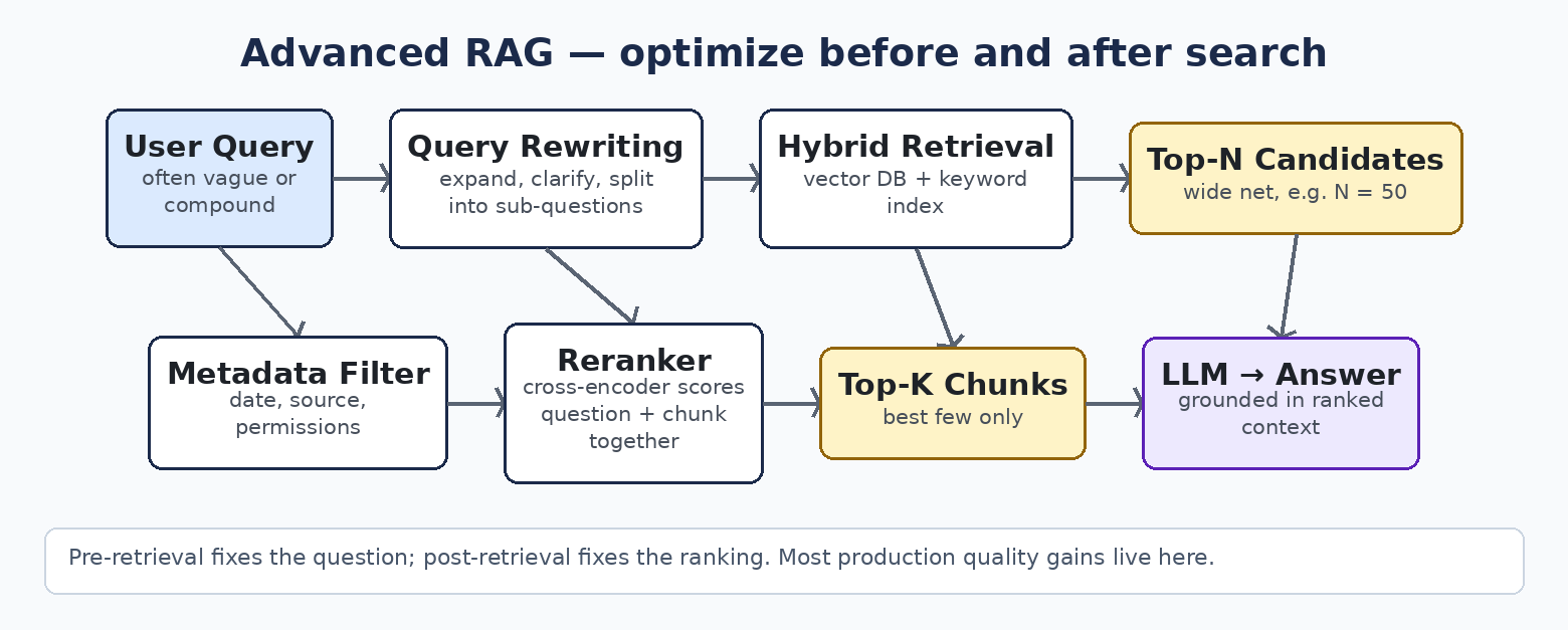
Reranking. A second, slower, more careful scoring pass. The vector search retrieves, say, 50 candidate chunks quickly and approximately; a reranker (often a cross-encoder model that reads the question and each chunk together) reorders them by true relevance and keeps the best few. Cheap retrieval for recall, expensive reranking for precision.
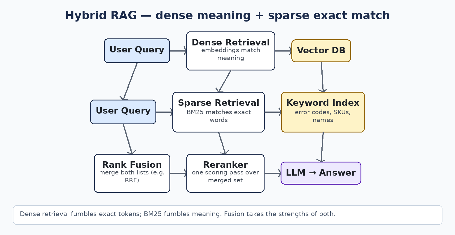
BM25. The classic keyword search algorithm — the technology behind decades of search engines. It matches actual words, weighted by rarity. Terrible at meaning, unbeatable at exact strings: error codes, part numbers, names, SKUs.
Dense vs. sparse retrieval. Dense = embedding-based (meaning). Sparse = keyword-based, like BM25 (exact words). Remember this pair; Hybrid RAG is just the two of them holding hands.
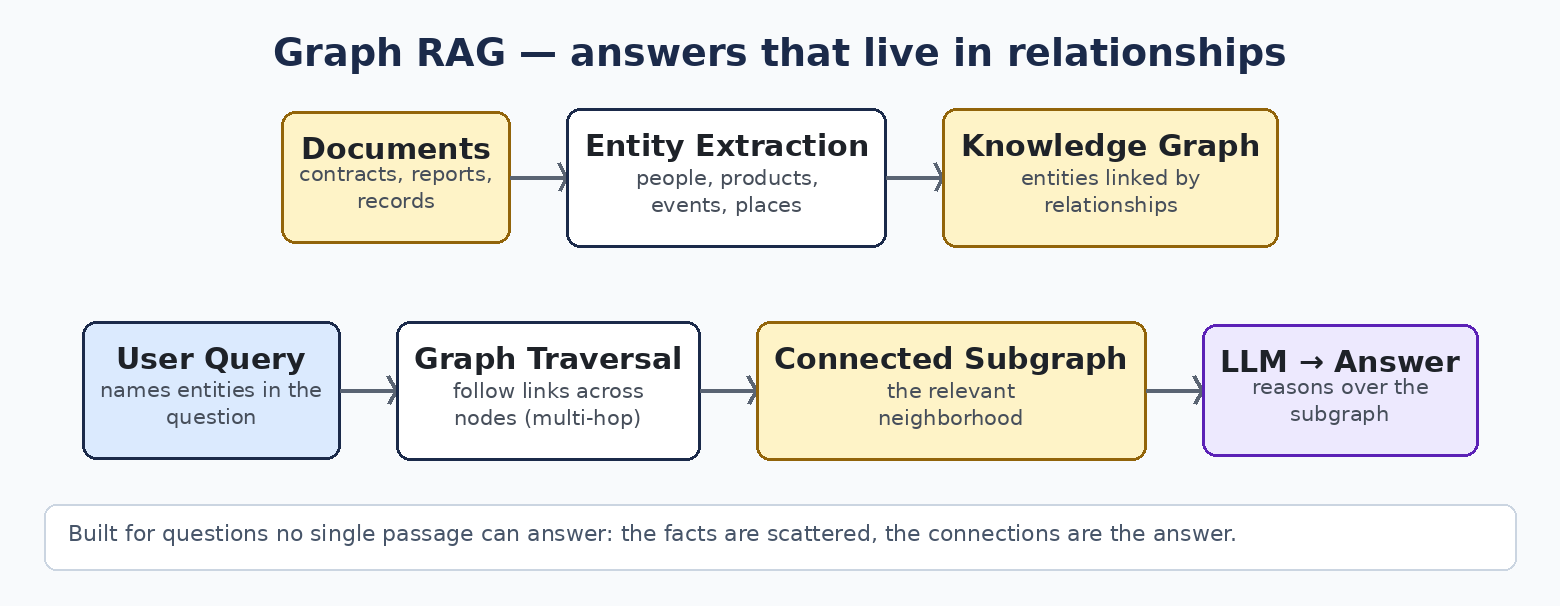
Knowledge graph. Information stored as entities and relationships — Customer → placed → Order → contains → Product — instead of as text chunks. You query it by traversal: following the links.
Grounding / faithfulness. Whether the answer is actually supported by the retrieved material, as opposed to the model improvising. The central quality question of every RAG system.
Hallucination. The model generating something fluent and false. In RAG, hallucination usually means the model answered beyond — or against — the context it was given.
Context window. How much text the model can consider at once, measured in tokens. Modern models offer 128K tokens and far beyond — which is what makes Long-Context RAG (type 9) possible at all.
With that in hand, the nine types will read easily.
1. Naive RAG — the baseline everything else improves on
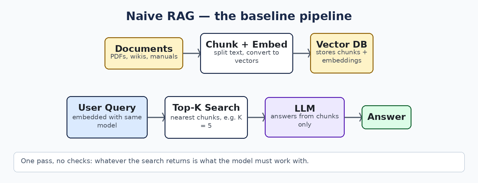
How it works. Documents are chunked, embedded, and stored in a vector database. A user question is embedded with the same model, the database returns the Top-K most similar chunks, those chunks are pasted into the prompt, and the LLM writes an answer from them. Four moving parts. You can build it in an afternoon.
When it earns its place. Internal document Q&A over a modest, well-behaved corpus. A proof of concept. Anywhere the questions are simple, the documents are the single source of truth, and “mostly right” is acceptable while you learn.
Where it breaks. Retrieval quality is the whole game, and naive retrieval is weak: chunk boundaries cut answers in half, the closest chunk by embedding is often not the chunk that answers the question, and there is no mechanism to notice failure. It retrieves once, blindly, and the model must make the best of whatever came back.
Say it in the interview. “Naive RAG is my starting point for any retrieval problem — it is the baseline you measure everything else against. I move beyond it the moment I can name the specific way retrieval is failing, because each advanced pattern exists to fix a particular failure.”
2. Advanced RAG — fixing retrieval before and after the search
How it works. Advanced RAG keeps the naive skeleton and wraps it with effort on both sides of the search. Before retrieval: the user’s question is rewritten (expanded, clarified, or split into sub-questions), because users ask badly and embeddings punish vague queries. After retrieval: results are filtered by metadata and reranked, so the model sees the best few chunks rather than the merely closest ones.
When it earns its place. When your naive system retrieves almost the right material — relevant documents exist, but the wrong passages surface. Complex or domain-specific corpora, where vocabulary is precise and questions are not. This is the single most common upgrade in production systems, because most RAG quality problems are retrieval problems wearing a disguise.
Where it breaks. Every added stage is latency and a tuning surface. A bad query rewrite can drag retrieval further from the answer than the original question would have. You now have knobs — rewrite strategy, filter logic, reranker choice, Top-K at each stage — and knobs demand evaluation, or you are tuning by vibes.
Say it in the interview. “Advanced RAG is pre-retrieval and post-retrieval optimization around the same core loop. Query rewriting fixes the question, reranking fixes the ranking. In my experience it is where the largest quality gains per dollar live.”
3. Modular RAG — RAG as interchangeable parts
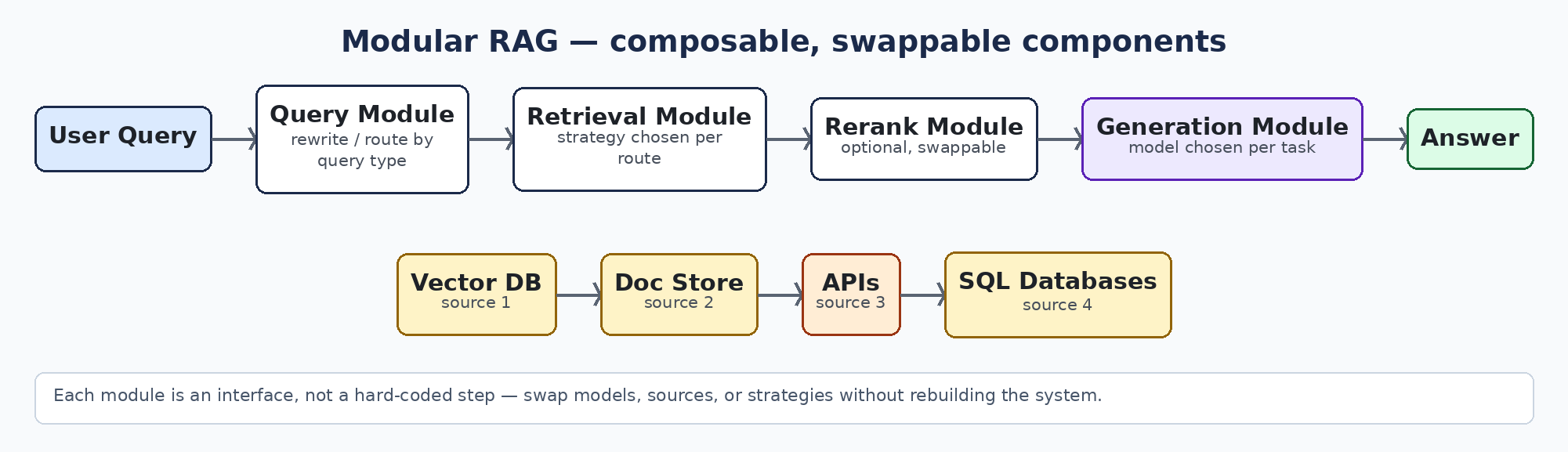
How it works. Instead of one fixed pipeline, the system is decomposed into modules — a query module, a retrieval module, a reranking module, a generation module — each swappable, each potentially backed by different sources: a vector database here, a document store there, an API or a SQL database alongside. Different queries can be routed through different combinations.
When it earns its place. Platforms, not features. When one team serves many use cases, when you need to experiment with components without rebuilding the system, or when different query types genuinely need different strategies. Modular RAG is less an architecture you choose on day one and more the shape a maturing system grows into.
Where it breaks. Abstraction is not free. You are now maintaining an orchestration layer, versioning components, and debugging interactions between parts that each look fine alone. For a single use case, it is engineering effort spent on flexibility you may never use.
Say it in the interview. “Modular RAG treats retrieval as composable services rather than a fixed pipeline. I reach for it when the system serves multiple use cases or sources — and I am honest that for one use case, it is over-engineering.”
4. Hybrid RAG — meaning and exact words, together
How it works. Run two retrievals in parallel: dense retrieval (embeddings) for meaning, and sparse retrieval (BM25) for exact keyword match. Merge the two result lists — typically with a fusion technique like Reciprocal Rank Fusion — then rerank the merged set and generate as usual.
When it earns its place. Anywhere exact strings carry meaning: error codes, product IDs, drug names, legal clauses, ticker symbols. Semantic search is famously blind here — an embedding will happily return text about a similar error code. BM25 will not. Real enterprise corpora are full of such strings, which is why hybrid is the quiet default in serious production systems.
Where it breaks. Two indexes to build, keep in sync, and tune. The fusion weighting between dense and sparse results is corpus-dependent, and the merged candidate set is bigger, so reranking cost rises.
Say it in the interview. “Embeddings match meaning but fumble exact tokens — SKUs, error codes, names. BM25 is the opposite. Hybrid retrieval runs both and fuses the rankings, and in enterprise data, where exact identifiers matter, it is usually my production default.”
5. Graph RAG — when the answer lives in the relationships
How it works. Instead of (or alongside) chunking text, you extract entities and their relationships into a knowledge graph. A question is answered by identifying the entities it mentions and traversing the graph — following relationships across nodes — then handing the connected subgraph to the model as context.
When it earns its place. Multi-hop questions: “Which suppliers provide components for the products that failed inspection last quarter?” No single document contains that answer; it exists only in the connections. Also for thematic questions over a whole corpus — “what are the main risk themes across these 500 reports?” — where chunk retrieval returns fragments but a graph can summarize structure.
Where it breaks. Somebody has to build and maintain the graph. Entity extraction is imperfect, relationships drift as data changes, and graph construction over a large corpus is a project in itself. If your questions are simple lookups, you have bought a very expensive way to avoid a vector search.
Say it in the interview. “Graph RAG answers questions whose answers live in relationships, not in any single passage. The cost is graph construction and upkeep, so I justify it with genuinely multi-hop questions — and I can point to the queries that chunk retrieval structurally cannot answer.”
6. Agentic RAG — retrieval that thinks in loops
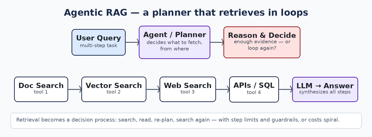
How it works. An AI agent — typically with a planning step — decides what to retrieve, from where, and whether it has enough. It can search documents, query a vector store, call web search, hit APIs, or run SQL, then reason about the results and loop: refine, search again, or answer. Retrieval stops being a single function call and becomes a decision process.
When it earns its place. Questions that need multiple steps and multiple sources: research tasks, investigations, anything where step two depends on what step one found. Also when the right source varies by question — no fixed pipeline can route as flexibly as an agent that reads the question and chooses.
Where it breaks. Everything compounds: latency (each loop is model calls), cost (same), and evaluation complexity (the path differs every run, so “why did it fail” becomes a forensic question). Agents also fail in agent ways — loops that never converge, tools called with malformed inputs, confident plans built on a misread first result. Guardrails and step limits are not optional.
Say it in the interview. “Agentic RAG replaces the fixed pipeline with a planner that chooses sources and iterates. It is the most capable pattern and the most expensive to run and evaluate, so I use it when the task genuinely requires multi-step reasoning over multiple sources — not as a default.”
7. Corrective RAG (CRAG) — retrieval that grades itself
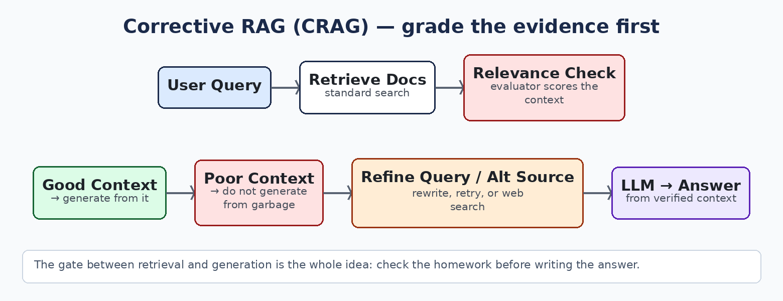
How it works. After retrieval, a lightweight evaluator scores the retrieved material for relevance before generation. Good context goes straight to the model. Poor context triggers corrective action — the query is refined and retrieval runs again, possibly against an alternative source such as web search. The system checks its own homework before answering. (From the CRAG paper, Yan et al., 2024.)
When it earns its place. When retrieval quality varies — mixed corpora, uneven document quality, questions that sometimes fall outside the knowledge base entirely. Also anywhere a wrong answer is expensive: if the context is bad, CRAG’s fallback beats generating from garbage and hoping.
Where it breaks. The evaluator is itself a model with errors; a relevance check that wrongly rejects good context adds cost and latency for nothing. The fallback path (web search, say) introduces its own trust questions. More components, more evaluation logic to validate.
Say it in the interview. “CRAG adds a relevance gate between retrieval and generation: score the context, and if it is poor, correct — rewrite the query, try another source — instead of generating from bad evidence. It is the pattern I choose when retrieval quality is uneven and wrong answers are costly.”
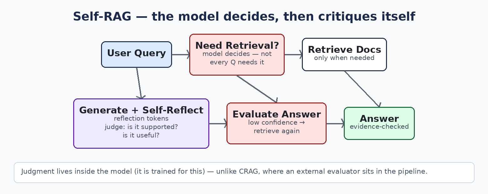
8. Self-RAG — the model decides whether to retrieve, then grades its own answer
How it works. Self-RAG (Asai et al., 2023) trains the model itself to control the process. The model first decides whether retrieval is even needed for this question. If it retrieves, it generates while critiquing its own output with special “reflection tokens” — judging whether passages support the answer and whether the answer is useful — and can retrieve again if its confidence is low.
When it earns its place. Mixed workloads: many questions the model can answer from its own knowledge, some that demand evidence. Retrieving for every question wastes cost and can actively hurt — irrelevant context drags good answers down. Self-RAG also shines where you want evidence-grounded generation with explicit self-checking built in, rather than bolted on.
Where it breaks. It requires a model trained (or fine-tuned) for the reflection-token scheme — you cannot bolt Self-RAG onto an arbitrary off-the-shelf model the way you can with CRAG. The extra critique steps cost tokens and time, and the quality of the whole loop depends on that specialized training.
Say it in the interview. “Self-RAG puts the control inside the model: it learns when to retrieve and how to critique its own generations using reflection tokens. The distinction from CRAG is where the judgment lives — in the model’s training versus an external evaluator in the pipeline.”
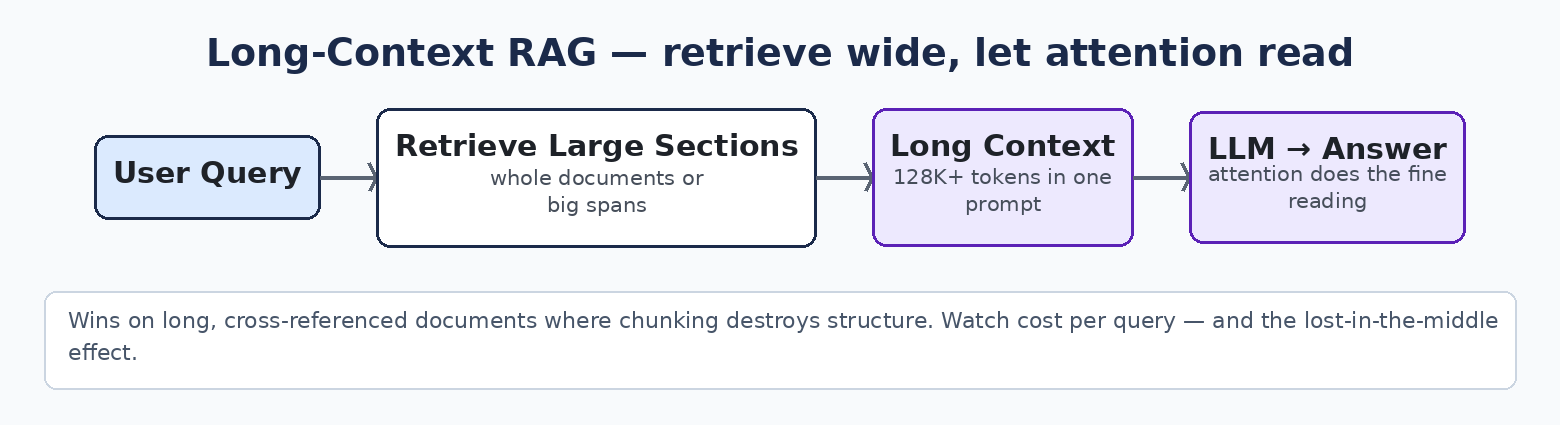
9. Long-Context RAG — when the window got big enough to skip the funnel
How it works. Modern models accept enormous inputs — 128K tokens and well beyond. Long-context RAG retrieves generously (large sections, or entire documents) and lets the model’s attention do the fine-grained work that chunking and reranking used to do. The retrieval funnel gets wider and shallower.
When it earns its place. Long, interconnected documents where answers span sections — contracts, clinical guidelines, regulatory filings — and chunking destroys exactly the cross-references that matter. Also small-to-medium corpora where “just put the relevant documents in the prompt” is honestly feasible.
Where it breaks. Inference cost scales with input, and a fat context on every query gets expensive fast. And a hard truth from practice: more context is not automatically better accuracy. Models can lose material in the middle of very long inputs, and irrelevant bulk dilutes attention. Retrieval still earns its keep as a cost and focus mechanism — long context changes the trade-off, it does not repeal it.
Say it in the interview. “Long-context models let me retrieve coarsely and let attention do the fine work. It wins on interconnected documents, but I watch cost per query and the lost-in-the-middle effect — bigger context is a trade-off, not a free upgrade.”
The decision guide
Start from the problem, not the pattern:
Your situation
Start with
Because
Simple document Q&A, small corpus, proving value
Naive RAG
Fastest path to a working baseline
Retrieval returns almost-right passages
Advanced RAG
Rewriting + reranking fix the ranking, cheaply
Exact codes, IDs, names matter alongside meaning
Hybrid RAG
Dense misses exact tokens; BM25 misses meaning; you need both
Questions connect entities across documents
Graph RAG
The answer is in the relationships, not any single passage
Multi-step questions spanning several sources/tools
Agentic RAG
A planner can route and iterate; a fixed pipeline cannot
Retrieval quality is uneven; wrong answers are expensive
Corrective RAG
Grade the evidence before you generate from it
Mixed workload; many questions need no retrieval
Self-RAG
The model learns when retrieval helps and when it hurts
Long, cross-referenced documents; modest corpus
Long-Context RAG
Chunking destroys the structure the answers depend on
Multiple use cases on one platform
Modular RAG
Composable parts beat one pipeline per use case
And the sentence that ties it together, in any interview room: these patterns compose. A production system might be modular in structure, hybrid in retrieval, corrective at the gate, and agentic for its hardest query class. The nine types are a vocabulary for decisions, not a multiple-choice question with one right answer.
FAQs
Q: Is RAG better than fine-tuning?
They solve different problems. Fine-tuning changes how the model behaves — tone, format, task skill. RAG changes what the model knows at answer time. If your problem is “the model doesn’t know our current data,” that is RAG. If it is “the model doesn’t follow our format,” that is fine-tuning. Serious systems often use both, and reaching for fine-tuning to inject facts is the classic beginner mistake — facts change, and retraining is a slow way to update them.
Q: What chunk size should I use?
There is no universal number, which is exactly why interviewers ask. Reasonable defaults are a few hundred tokens with some overlap between chunks, but the honest answer is: it depends on the document structure and the questions, and you decide by evaluating retrieval quality on real queries, not by folklore. Structure-aware chunking (splitting on headings, keeping tables intact) usually beats any magic number.
Q: How do I know if my RAG system is actually good?
Evaluate the two halves separately. Retrieval: are the right chunks coming back (recall and ranking quality against a set of real questions with known answers)? Generation: is the answer faithful to the retrieved context, and does it actually address the question? Teams that only eyeball final answers cannot tell which half is failing — and it is usually retrieval.
Q: Vector database — which one should I pick?
For most teams, the honest answer is: the one that fits your existing stack and scale, because at moderate scale they are more alike than different. The decision matters more at very large scale, with heavy metadata filtering, or with hybrid search requirements. In an interview, talk about the criteria — scale, filtering, hybrid support, operational burden — not brand loyalty.
Q: Doesn’t long context make RAG obsolete?
No — it reprices it. Stuffing everything into the prompt costs more per query, slows responses, and can reduce accuracy when relevant material sits buried mid-context. Retrieval remains how you control cost and focus attention. What long context changes is granularity: you can retrieve documents instead of fragments and let the model read widely within a selected set.
Q: When should I NOT use RAG at all?
When the knowledge is tiny and static (put it in the prompt), when the task needs no external facts (pure reasoning or transformation), and when the real problem is structured transactions — if the user needs the current account balance, that is a database query or a tool call, not a document search.
Q: How do I stop a RAG system from answering questions it has no evidence for?
Teach it to abstain. Instruct the model to answer only from context and to say so when the context is insufficient, evaluate faithfulness, and consider a corrective pattern (CRAG) that detects poor retrieval before generation. A system that says “I don’t have that in the knowledge base” is worth ten that improvise.
Q: What’s the difference between CRAG and Self-RAG?
Where the judgment lives. CRAG puts an external evaluator in the pipeline — any model can sit behind it. Self-RAG builds the judgment into the model itself through training with reflection tokens. CRAG is easier to adopt; Self-RAG is more integrated but requires the specialized model.
Interview rapid-fire
“Walk me through how you’d design a RAG system for [our documents].”
Start with the naive baseline and say so. Then ask (or state assumptions) about corpus size, question types, exact-match needs, and cost of a wrong answer — and let those answers pull in advanced, hybrid, or corrective patterns one at a time, naming the failure each addition fixes. This structure — baseline, then failure-driven upgrades — is the strongest signal you can send.
“Our RAG system hallucinates. What do you check first?”
Whether the retrieved context contained the answer at all. Most “hallucination” in RAG is retrieval failure followed by the model filling the gap. Check retrieval quality on the failing questions before touching prompts or models.
“Why not just use a bigger model?”
A bigger model reasons better over the context it is given; it does not fix being given the wrong context, and it multiplies cost across every query. Architecture first, model size second.
“How would you cut our RAG costs?”
Retrieve less but better (reranking lets you shrink Top-K), cache frequent queries and embeddings, route simple questions to smaller models, and reserve agentic or long-context patterns for the query classes that demonstrably need them.
The one-sentence version
RAG is not a product you install; it is a set of decisions about how evidence reaches the model — and the right architecture is the simplest one whose failure modes you have actually observed and priced.
Start simple. Measure. Add exactly the complexity your failures demand. That sentence will carry you through most interviews — and, not coincidentally, most production systems too.
If this helped, subscribe to The Agentic Enterprise below — one practical AI architecture breakdown a month, written from production experience, no hype. And if you are preparing for interviews, the free GenAI Interview Question Bank on the Free Toolkits page goes deeper.
In the earlier piece on the semantic layer, I made the case: define each business metric once, and let every dashboard, tool, and AI agent read from it. This is the hands-on companion. We build one.
What we’re building: a metrics layer for a single metric — revenue — that your BI tool, your dbt project, and an AI agent can all consume without disagreeing. By the end, “revenue” means one thing everywhere, it’s tested, and it’s served through an API.
Step 1: Define the metric with a human, not in YAML
The unsexy step that decides everything. Before touching code, get the business owner in a room (or a doc) and nail down:
Name: revenue Definition: gross revenue, refunds excluded, recognized on order date Grain: one row per day per region Owner: who signs off when the number looks wrong
Write this down where everyone can see it. Most metric disagreements I’ve seen weren’t technical — two teams with two definitions, both convinced theirs was “revenue.” The semantic layer doesn’t fix disagreement. It forces the conversation early, once, instead of late, forever.
Step 2: Model it
Here’s the shape of a semantic model in dbt’s MetricFlow format (adapt to your dbt version — the concepts transfer to any tool):
semantic_models:
  - name: orders
    description: Order-level facts, one row per order line
    defaults:
      agg_time_dimension: ordered_at
    entities:
      - name: order_id
        type: primary
      - name: customer_id
        type: foreign
    dimensions:
      - name: ordered_at
        type: TIME
        type_params:
          time_granularity: day
      - name: region
        type: CATEGORICAL
    measures:
      - name: order_total
        agg: SUM
        expr: line_total

metrics:
  - name: revenue
    description: Gross revenue, refunds excluded, recognized on order date
    type: SIMPLE
    type_params:
      measure: order_total
Three things to notice. First, the measure (order_total) is the raw aggregation; the metric (revenue) is the business concept layered on top with its definition. Second, dimensions like region and ordered_at are what let every consumer slice the same metric the same way. Third, the description isn’t decoration — it’s the contract. When an AI agent reads this metric, the description is what keeps it from inventing its own interpretation.
No dbt? A SQL view gets you 80% of the way:
CREATE OR REPLACE VIEW marts.revenue_daily AS
SELECT
  DATE_TRUNC('day', ordered_at) AS day,
  region,
  SUM(line_total) AS revenue
FROM orders
WHERE order_status != 'refunded'
GROUP BY 1, 2;
Same idea: one definition, one place, everyone reads from it.
Step 3: Test it like production code
Metrics without tests are rumors. At minimum:
Sanity bounds: revenue is never negative; day-over-day change beyond some threshold pages someone. Grain checks: no duplicate day/region rows; no future dates. Reconciliation: the semantic layer’s revenue matches the finance system’s revenue within tolerance, on a schedule.
In dbt, these are data tests on the underlying models plus a scheduled reconciliation query. The point isn’t the tooling — it’s the discipline. A metric nobody tests is a metric nobody trusts, and an untrusted metric gets forked: someone builds their own version in a spreadsheet, and you’re back to three definitions of revenue.
Step 4: Serve it to everyone — including agents
This is the step most teams skip, and it’s the whole point.
Your BI tool connects to the semantic layer natively (most modern BI tools speak dbt’s Semantic Layer or query the views directly). But the second consumer — the AI agent — needs the same metrics through an API, not a dashboard. The agent should ask for “revenue by region for Q3” by metric name and get back a governed number, not write its own SQL against raw tables and reinvent the definition.
That’s the real payoff: the agent stops hallucinating metrics because it stops computing them. It reads them.
Step 5: Govern changes
Metrics change. Tax rules change, refund policies change, someone acquires a company. The semantic layer needs change control like any production system:
Versioning: metric definitions are versioned; breaking changes get a migration path, not a silent edit. Ownership: every metric has an owner who approves changes. No owner, no metric. Deprecation: old definitions get sunset with notice, not deleted on a Friday.
Humans grumble at schema changes and adapt. Agents break silently. Versioning isn’t bureaucracy — it’s the difference between a controlled rollout and a fleet of agents confidently reporting last quarter’s definition.
Five mistakes I see everywhere
1. Defining metrics in the BI tool. Now your definition lives in one vendor’s dialect, invisible to everyone else — including your agents. The semantic layer belongs underneath the BI tool, not inside it.
2. No owner per metric. A metric nobody owns is a metric nobody fixes. Assign ownership on day one.
3. Grain ambiguity. Is revenue recognized on order date or ship date? If the model doesn’t say, every consumer guesses — differently.
4. Skipping tests. “Trust me” is not a data quality strategy. Test the metric, reconcile it against finance, alert on drift.
5. Letting teams fork definitions. The moment someone builds “revenue_v2_final_FINAL” in a spreadsheet, you’ve lost. Make the governed path the easy path: good docs, fast queries, one API.
The payoff
A working semantic layer is unglamorous. No demo has ever wowed a room with “consistent metric definitions.” But it’s the foundation everything else stands on: dashboards people trust, agents that don’t invent numbers, and executives who stop arguing about whose report is right.
Build it once, define it once, test it, serve it to everyone. The iceberg below the waterline holds up the tip.